It’s summer. You’re heading back home after an evening at the beach. Looking out of the car window, bored, you tune into the radio. It’s been so long. Listening to this old recording, you can’t even recall exactly when it was.

Submit the date and time of the recording in the format toh{DD-MM-YYYY-HH-MM}. The time should be provided in the local time zone where the audio was recorded.

Hint: The answer isn’t in the file metadata.

Description

You are given an audio file called summer.m4a. The task is to determine the date and time of the recording based on the content of the audio.

The audio was recorded in a car from the radio. It plays music that is a periodic interlude for Rai Radio 1, the top Italian public radio channel. The music is a jingle that plays every hour, and it is followed by a time signal that tells the current time in a coded format.

For international players who may not be familiar with this, it was sufficient to realize that what was playing was a time signal and hear the words “Rai Radio 1”, which can be heard at the start of the clip. By simply searching things like “Rai Time Signal” on Google, it is possible to find a variety of links detailing the structure of the time signal and how to decode it.

Other examples of such transmission can be found on YouTube, such as this one:

Historical Context

Between 1979 and 2016, the italian national television and radio broadcast company (RAI) used to broadcast the exact time from the atomic clock of the INRiM, the national institute of metrologic research. After the 31st of December 2016, INRiM exact time stopped being broadcast by radio, in favour of the more efficient and precise Network Time Protocol syncronization. The time signal as of 2022 is still broadcast on Rai Radio 1 for nostalgia purposes, but isn’t used to sync devices anymore.

Time Signal Structure

The following is a diagram that I remastered and translated to English from the original source.

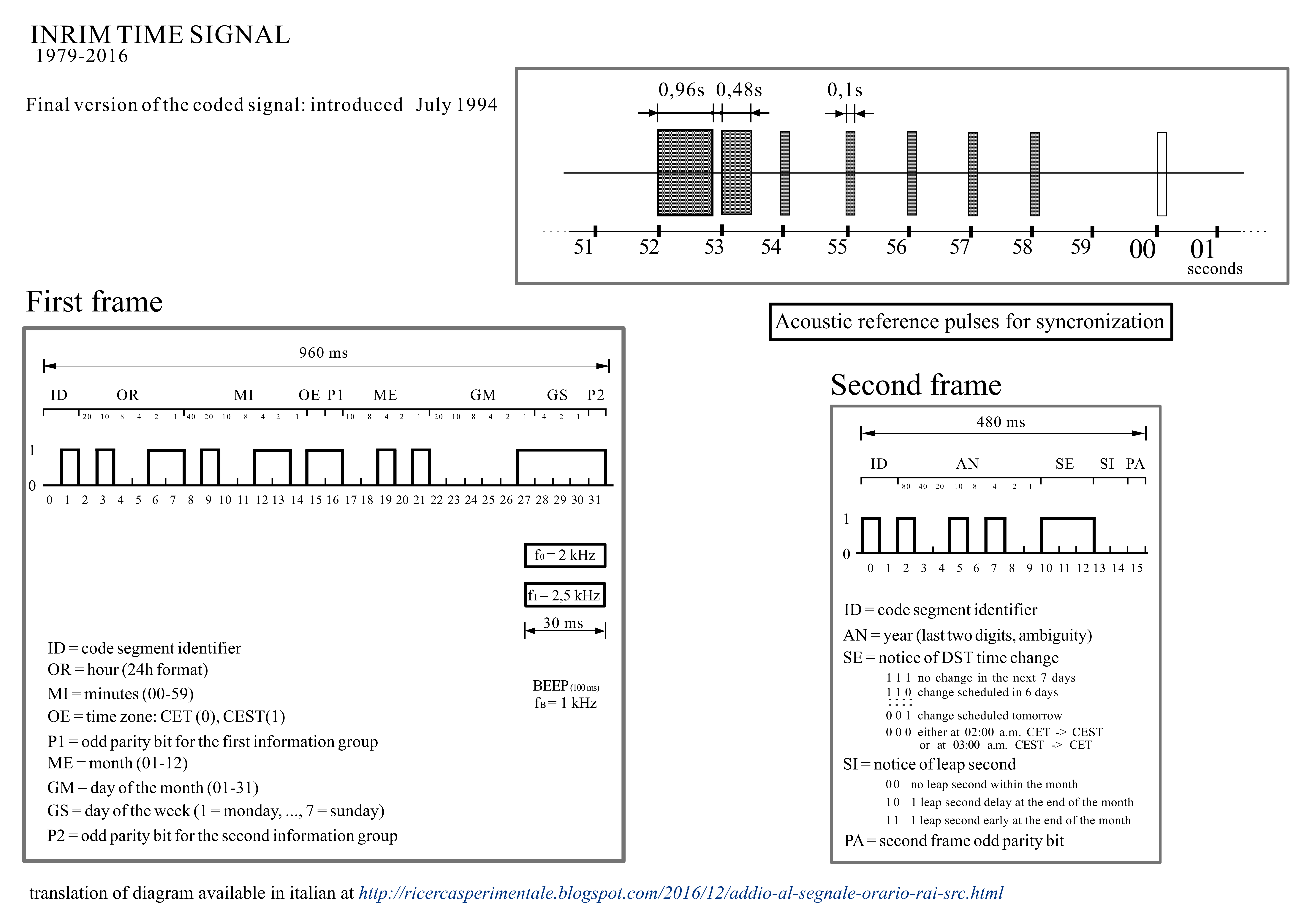
If the signal was clean, it would be straightforward to decode the content. However, the audio has been recorded on the road and there are even sounds of the car’s turning signals.

Luckily, we know the information in the time signal frames is encoded with Frequency Shift Keying (FSK). That is, the signal is modulated by two different frequencies, one for the “0” bit and one for the “1” bit. 0 corresponds to 2kHz and 1 corresponds to 2.5kHz. The duration of each bit is 30 ms. We can start by filtering the audio to isolate the two frequencies with a bandpass filter.

import numpy as np
import matplotlib.pyplot as plt
import wave
from scipy.signal import butter, sosfiltfilt, sosfreqz

# ------------------------------------------------------------------
# 1. parameters you may want to tweak
# ------------------------------------------------------------------
wav_path   = "./signal.wav"      # path to your file
f1, f2     = 2000, 2500          # centre frequencies (Hz)
bw         = 200                 # full bandwidth (Hz)  ⇢  ±bw/2 either side
filter_order = 8                 # 8-pole Butterworth
samples_to_show = 44100 * 5      # 5 s of waveform in the plot
# ------------------------------------------------------------------

def bandpass(signal, centre, bw, fs, order=8):
    """
    Zero-phase Butterworth band-pass using second-order sections.
    centre : centre frequency in Hz
    bw     : full bandwidth in Hz   (pass-band = centre ± bw/2)
    """
    low  = centre - bw/2
    high = centre + bw/2
    sos  = butter(order, [low, high], btype='bandpass',
                  fs=fs, output='sos')
    return sosfiltfilt(sos, signal)

# ------------------------------------------------------------------
# open WAV, extract mono float signal
# ------------------------------------------------------------------
with wave.open(wav_path, 'rb') as wf:
    n_channels   = wf.getnchannels()
    sample_width = wf.getsampwidth()
    fs           = wf.getframerate()
    n_frames     = wf.getnframes()
    print(wf.getparams())

    audio_bytes  = wf.readframes(n_frames)

# inter-leaved int16 → mono float32 in [-1,1]
signal = np.frombuffer(audio_bytes, dtype=np.int16).reshape(-1, n_channels)
signal = signal.mean(axis=1).astype(np.float32) / 32768.0

# ------------------------------------------------------------------
# filter
# ------------------------------------------------------------------
filtered1 = bandpass(signal, f1, bw, fs, order=filter_order)
filtered2 = bandpass(signal, f2, bw, fs, order=filter_order)

# ------------------------------------------------------------------
# quick frequency-response sanity check (optional)
# ------------------------------------------------------------------
w, h = sosfreqz(
    butter(filter_order,
        [f1-bw/2, f1+bw/2],
        btype='bandpass', fs=fs, output='sos'),
worN=4096, fs=fs)

Then, to plot the result:

plt.figure(figsize=(6,4))
plt.semilogx(w, 20*np.log10(np.abs(h)))
plt.title(f'{filter_order}-pole band-pass {f1-bw/2:.0f}–{f1+bw/2:.0f} Hz')
plt.xlabel('Frequency (Hz)'); plt.ylabel('Magnitude (dB)')
plt.grid(True, which='both', ls=':')
plt.tight_layout()
plt.show()

# ------------------------------------------------------------------
# time-domain plot (first few seconds)
# ------------------------------------------------------------------
time = np.arange(len(signal)) / fs

fig, axs = plt.subplots(2, 1, figsize=(12, 8), sharex=True)

axs[0].plot(time[:samples_to_show], signal[:samples_to_show],
            color='0.6', lw=0.7, label='Original')
axs[0].plot(time[:samples_to_show], filtered1[:samples_to_show],
            label=f'Filtered {f1-bw/2:.0f}-{f1+bw/2:.0f} Hz')
axs[0].set_ylabel('Amplitude')
axs[0].set_title('Band-pass around {:.0f} Hz'.format(f1))
axs[0].legend()

axs[1].plot(time[:samples_to_show], signal[:samples_to_show],
            color='0.6', lw=0.7, label='Original')
axs[1].plot(time[:samples_to_show], filtered2[:samples_to_show],
            label=f'Filtered {f2-bw/2:.0f}-{f2+bw/2:.0f} Hz')
axs[1].set_ylabel('Amplitude')
axs[1].set_xlabel('Time (s)')
axs[1].set_title('Band-pass around {:.0f} Hz'.format(f2))
axs[1].legend()

plt.tight_layout()
plt.show()

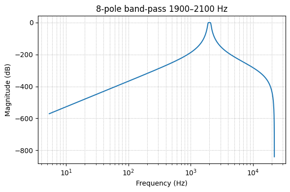
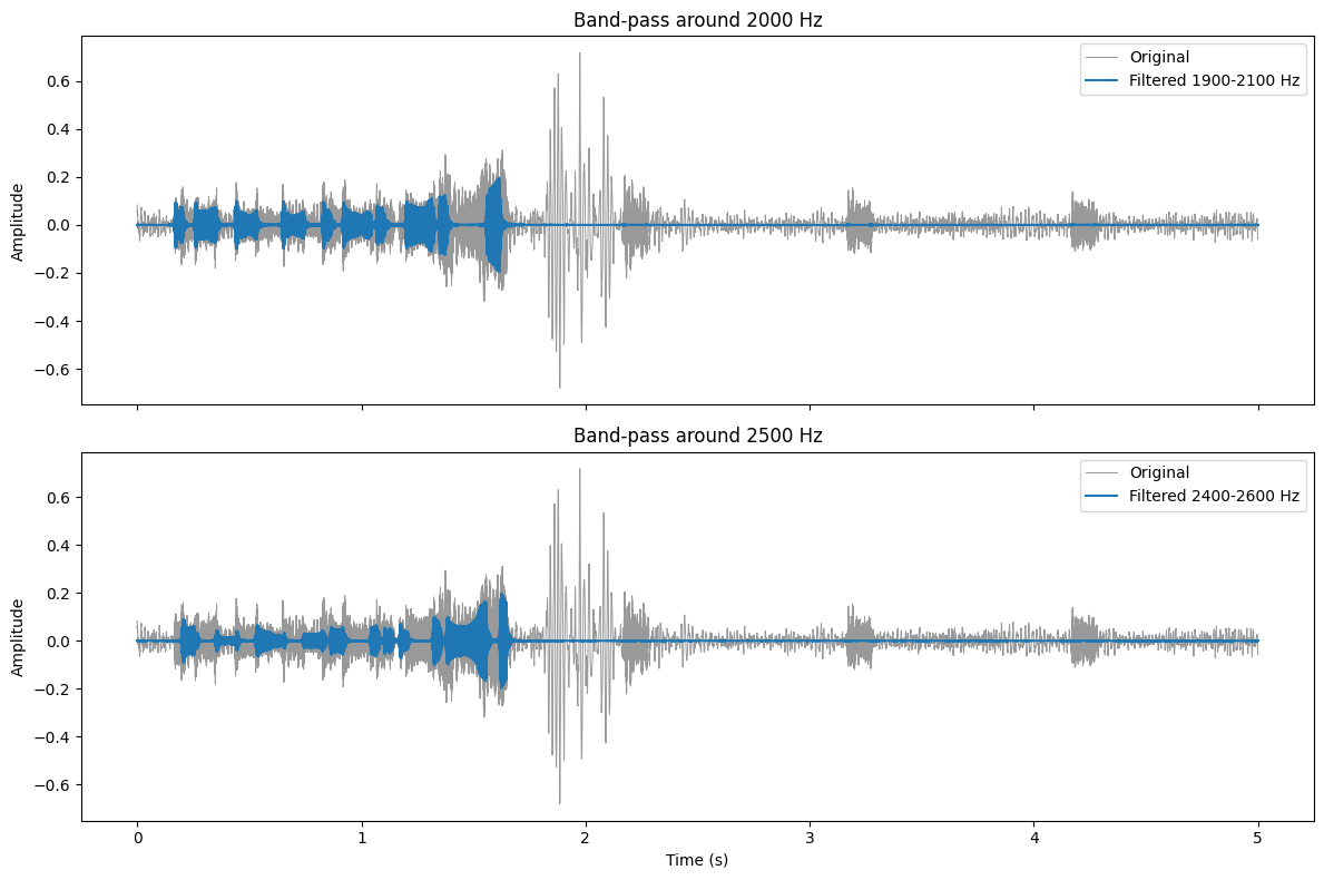
This is not very easy to visualize in detail, so let’s try to highlight the two frequencies with different colors.

# Show the first 2 seconds of both filtered signals together
samples_to_show = 44100 * 2  # 2 seconds
grid_interval_ms = 30  # 30ms grid lines
grid_interval_samples = int(grid_interval_ms / 1000 * fs)
grid_start_ms = 10  # Start position of first grid line (in ms)

plt.figure(figsize=(14, 6))
time = np.arange(samples_to_show) / fs  # time in seconds for x-axis

# Plot both filtered signals
plt.plot(time, filtered1[:samples_to_show], 
         color='blue', lw=1.2, alpha=0.8, 
         label=f'Band-pass {f1-bw/2:.0f}-{f1+bw/2:.0f} Hz')
plt.plot(time, filtered2[:samples_to_show], 
         color='green', lw=1.2, alpha=0.8, 
         label=f'Band-pass {f2-bw/2:.0f}-{f2+bw/2:.0f} Hz')

# Add vertical grid lines every 30ms, starting from grid_start_ms
grid_positions = np.arange(grid_start_ms/1000, time[-1], grid_interval_ms/1000)
for pos in grid_positions:
    plt.axvline(x=pos, color='red', linestyle=':', alpha=0.5, linewidth=0.8)

# Add labels and legend
plt.xlabel('Time (s)')
plt.ylabel('Amplitude')
plt.title('Comparison of Band-pass Filtered Signals (2 seconds)')
plt.legend(loc='upper right')
plt.grid(True, which='major', axis='y', alpha=0.3)
plt.tight_layout()
plt.show()

This plot shows the signal intensities colored by frequency. The blue line represents the 2kHz signal, and the green line represents the 2.5kHz signal. The red vertical lines indicate the 30ms intervals where the bits are transmitted.

The small numbers in each bit of multi-bit blocks correspond to values that should be summed to form the final value. For example, in the reference of the structure, the value of the Hour is 10 + 2 + 1 = 13, whereas the value of minutes is 20 + 4 + 2 = 26 which corresponds to 1:26 PM

Parity computation is odd, which means that the parity bit is 1 if the number of 1s in the frame is odd, and 0 if it is even.

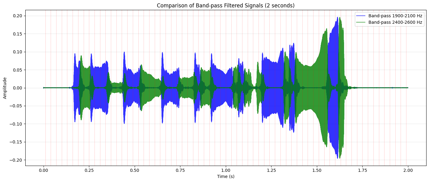
Since the signal is noisy, we need to reason on what we have. Some values of bits will be likely to be correct (when adjacent bits are the same), while others will have a degree of uncertainty (when adjacent bits are different).

1. First, the first two bits of each frame are always the same (code segment identifiers). As such, we know that for a well-formed frame, the first two bits should be “01”. The start of the second frame is instead always “10”.

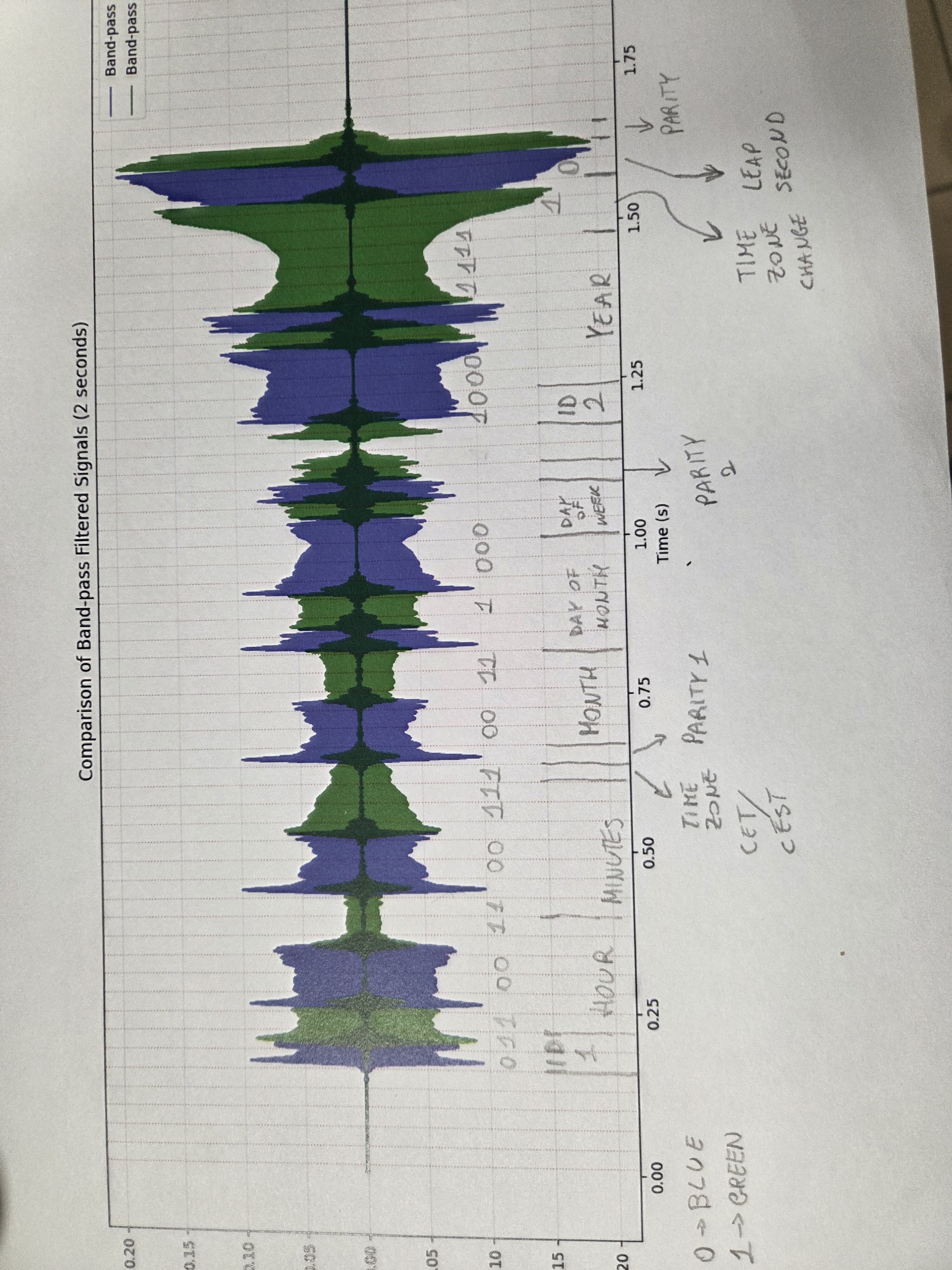
2. At the same time, we can proceed to pin values of bits where no change occurs (high confidence bits).

3. Minutes are 40 + x + 2 + 1. x cannot be 20, as it would exceed the maximum value of 59. So, the bit corresponding to 20 is 0. Thus, the value of minutes can either be 43 or 47. Let’s leave it in doubt for now.

4. We can do a similar reasoning for the hours. Given the confident bits, the bit corresponding to 10 must be 0 (the 20 bit is surely 1). As such, the hour can either be 21 or 23.

5. The time zone is surely CEST (UTC+2), because the bit is in a high confidence zone of 1.

6. P1 looks like is more likely to be 1 than zero. In fact, even though it is mixed, there is a clear peak for the frequency of 2kHz. Since parity is odd, we need the sum of bits (including parity) to be odd. The value of P1 is 0, so the number of preceding 1s is even. This means remaining bits will need to have the same value. Either both are 0 or both are 1.
   
   This means the time was either 21:43 or 23:47.

7. Month is either 3 or 7 (March or July). Looking at Italian Leap second history on Google, we can see they either happen in June or December. So the bits for leap second are all 0s (no leap second).

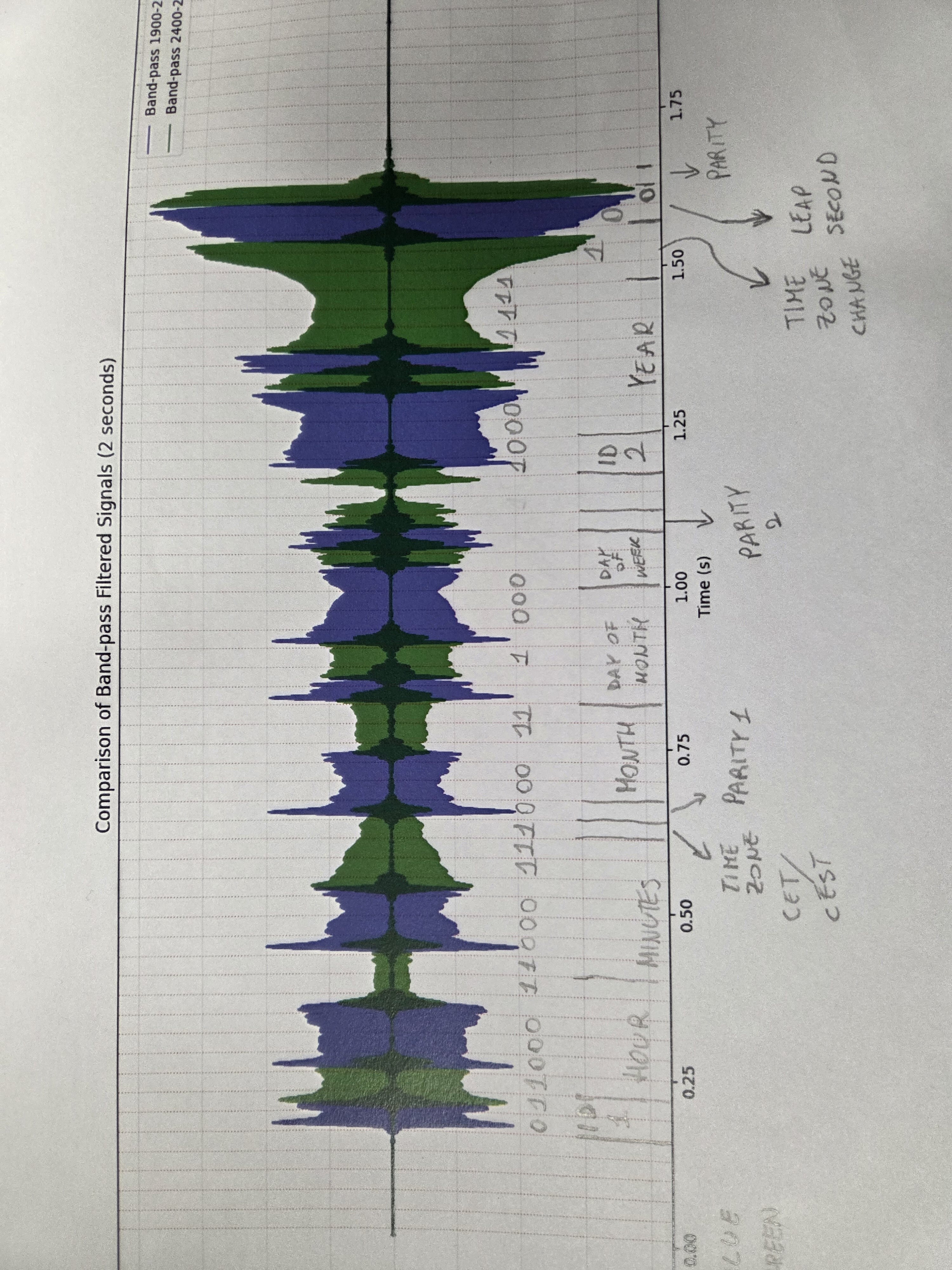
8. Looking at the sharp transition between the bit for 10 and 8 of the Year, we can tell that it’s likely they are a 1 and a 0 respectively. This means the year is x + 10 + 4 + 2 + 1 = either 2017 or 2037. The challenge mentions nostalgia for the past, not looking forward to the future, so we can assume the year is 2017.

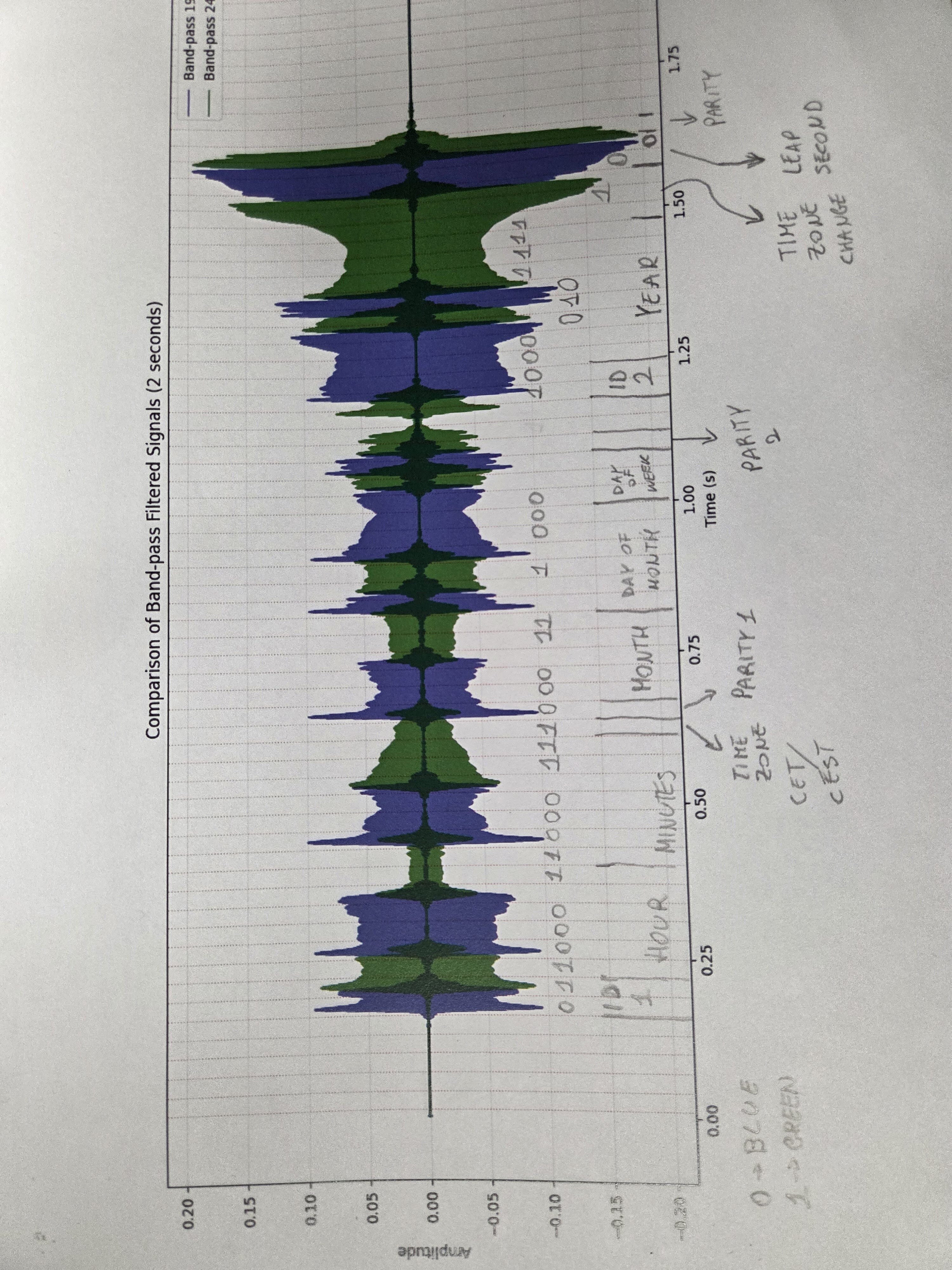
9. Now in the second frame we are just missing the parity bit and the last bit for the Time Zone change. The parity bit is likely one, since the signal ends with a 2.5kHz tail. So the sum of bits (including parity) is odd. The time zone change bit is likely 0, since the signal ends with a 2.5kHz tail. We already have 7 bits of 1s, so the remaining bit must be 1 to make the total number of 1s odd.

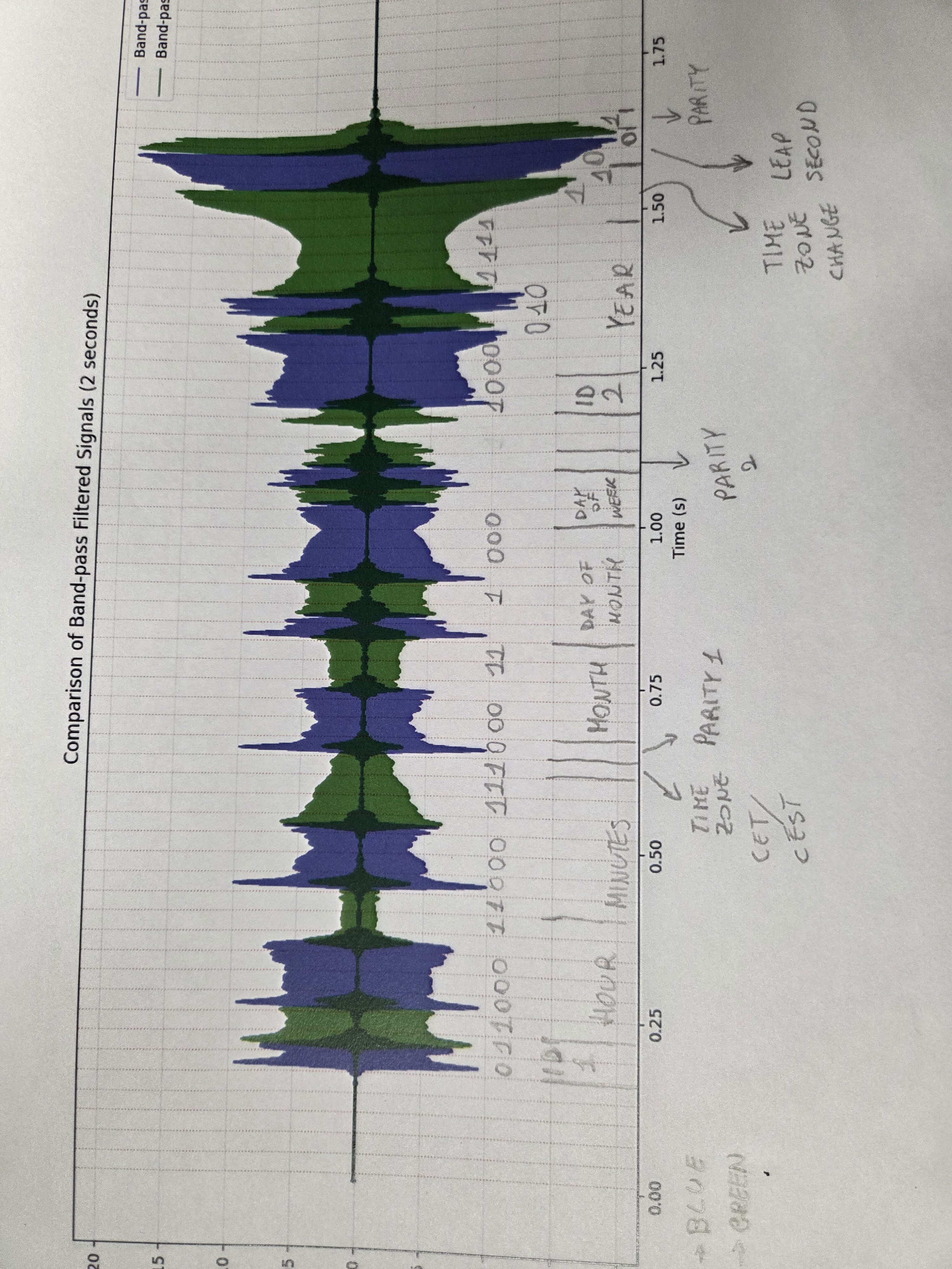
10. The Time Zone Change block is 111, which means no change in time zone is scheduled for the next 7 days. Again, searching on Google, we can see that in 2017 the time zone changed from CET to CEST on March 26 and from CEST to CET on October 29. Possible days of the month with bits we have pinned are 8, 12, 18, 22, 28. If this is March, we can only have the 28th (it is already summer time), otherwise, we can have any the above. Given the shape of the peaks, the most likely is th 18th. As such, it’s unlikely to be March, so we can assume the date is July 18th. This assumption would fit with the transition we have in the block that indicates the day of the week, which looks to be a 2 (Tuesday). July 18th, 2017 was a Tuesday.

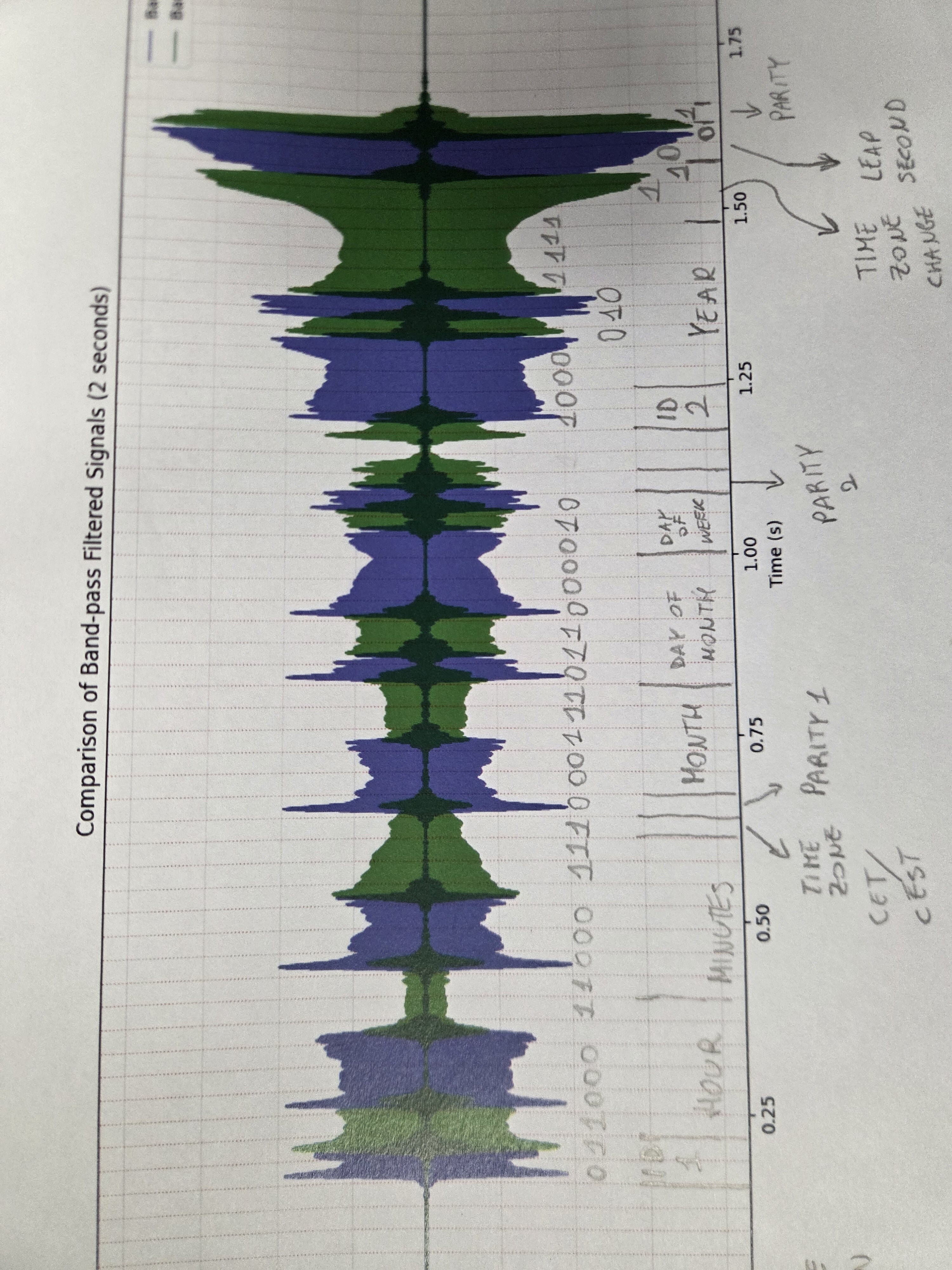
11. Finally, we break the last assumption. Between the two remaining bits, the one in the Hours and the one in the Minutes, the one in the Hours is less uncertain. It looks like the 2.5kHz signal, while less intense, is mounting right at the start of the 30 ms block. On the contrary, the 2kHz signal is clearly decreasing during the block. That being the case, both bits are likely 1, which means the time is 23:47.

Thus, the final information block is 01100011100011110001110110000101 1000010111111001

Date Tuesday July 18 2017 23:47 CEST

Thus, the flag is toh{18-07-2017-23-47}.

To read more about the INRiM time signal, as well as a working python implementation of the encoder and (more or less) decoder, you can check out my pyRAIsrc, which was made private during the CTF to avoid OSINTs, but is now public again.